The solar industry is often referred to as the “solar coaster” due to its seemingly constant changes as equipment manufacturers innovate, permitting requirements fluctuate, electrical codes update, and new policies become mandate. But, like in any industry, some unwritten rules find a way to stand the test of time. In this article we will analyze one of those, the 2% DC voltage drop assumption, to see if it’s still pertinent to PV projects today.
What is the 2% voltage drop rule?
In the solar industry lexicon, 2% voltage drop has been known to system integrators as a hard rule that, when sizing conductors, the DC voltage drop should be limited to no higher than 2%. When pushed to explain why, nearly everyone answers with some form of “That’s how it’s always been done.”
While a firm 2% DC voltage drop rule is not formally written in code anywhere, it should be noted that the National Electrical Code (NEC) sections 210.19(A) Informational Note 4 (below) and 215.2(A) Informational Note 2 do recommend that voltage drop be limited in certain scenarios. Subsequent references in the Code refer back to these notes as if they were established code requirements. The only sections of code that explicitly call for voltage-drop limit are for specific sensitive or emergency equipment such as sensitive electronic equipment (NEC 647.4(D)), fire pumps (NEC 695.7), and energy storage cell terminal requirements (NEC 706.31(B)). Note that none of these special applications will apply to a typical PV system.
***
NEC Informational Note No. 4:
Conductors for branch circuits as defined in Article 100, sized to prevent a voltage drop exceeding 3 percent at the farthest outlet of power, heating, and lighting loads, or combinations of such loads, and where the maximum total voltage drop on both feeders and branch circuits to the farthest outlet does not exceed 5 percent, provide reasonable efficiency of operation. See Informational Note No. 2 of 215.2(A)(1) for voltage drop on feeder conductors.
***
Anecdotally, the rule’s origins trace back to the early days of PV installations, when modules were far more expensive and low-voltage systems were far more common. Lost voltage means lost power, and with high module prices, spending a little more money on larger-gauge wire to avoid losing very expensive power made a lot of sense (and cents). Additionally, with fewer modules in each series string, the potential for strings to drop out of the operating voltage window of the downstream inverter was of great concern. Therefore, an emphasis on voltage drop was justified to improve the overall production and operation of a PV array.
But it’s rare for such an assumption to hold true for multiple decades–especially in an industry that has shown it can dramatically change every few years–so let’s analyze the modern-day relevance of the rule and see if there is a better alternative based on today’s assumptions.
Modeling & Analyzing Voltage Drop in 2015
We should note that this is not our first analysis of the 2% DC voltage drop rule. In 2015, we sought to challenge its validity, concluding in a SolarPro magazine article that DC voltage drops based on standard test conditions (STC) didn’t hold true for real-world systems and performance.
Our 2015 analysis was based on a series of Helioscope models. To account for the vast difference in climates across the U.S., we built test sites in cities that are representative of high, medium, and low-irradiance (Phoenix, Atlanta, and Seattle) where we modeled 600V and 1000V systems using components that were consistent with the times: 305W modules with a 550kW central inverter(s).
Once our models were built, we simulated a year’s worth of production in the form of an “8760” spreadsheet, which we then analyzed in Excel to manually calculate and monetize the DC voltage drop at each site. Note: “8760” refers to the number of hours in a calendar year. The 8760 spreadsheet uses system parameters and historical weather data to estimate hourly production for a typical meteorological year at that given location.
This distinction–using real hourly data vs. nameplate equipment specifications and standard testing conditions–was vital to our analysis. By looking at actual hour-by-hour data, we could reliably claim that our voltage drop calculations were representative of real-world conditions. And consider what hours DC voltage drop actually is of concern. The equation we used to calculate static voltage drop for PV module strings was as follows:
Where VD% is the voltage drop percentage, L is the one-way circuit length (length from module string to connection point); I is the module operating current; R is the conductor resistance (at 75 degrees C); and Vsource is the voltage of the power source (the string of PV modules) at STC.
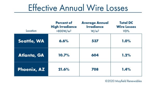
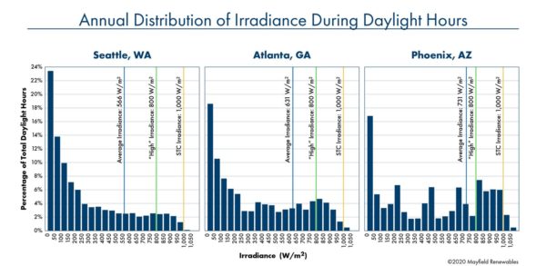
For comparison, a simpler and more common approach is to use the module maximum power voltage and maximum current values at STC (which assumes 25 degrees C cell temperature and 1000W/m2 irradiance). While this method is simpler to use in practice, its outputs tend to be more conservative than our voltage drop calculations using modeled data corrected for weather conditions. This is because, unsurprisingly, standard testing conditions are not indicative of real-world conditions. Our models found that, even in sunnier climates like Phoenix, only 21.6% of sun-hours had high-intensity sunlight of irradiance greater than 800W/m2. This effect becomes more pronounced in colder, more overcast cities like Seattle, with a paltry 6.6% of high-intensity sun-hours and where the average irradiance is just 537W/m2–half of the irradiance used in STC-based calculations. Based on differences in site temperature and irradiance alone, we found effective DC wire losses to be between 1% (in Seattle) and 1.4% (in Phoenix)–far lower than the assumed 2%.
As higher system voltages (in 2015, that meant up to 1000V) and inverter-load ratios (ILRs, also referred to as DC-to-AC ratios) were adopted more and more over time, the chasm between the assumed 2% voltage drop and real-world effective voltage drop widened further. Holding everything else constant, the voltage increase in the denominator of our voltage-drop equation will lower the percent voltage drop. And with higher ILRs, there is more opportunity for the system to overproduce on the DC side, otherwise known as a case of “power limiting” (or “power clipping”). In these cases, we may have voltage loss, but if the system is already shedding excess DC power, those losses do not matter. Comparing these losses to the losses during hours where the system is producing, but not power limiting, can give a real sense of the effect of voltage drop.
Modeling & Analyzing Voltage Drop in 2020
To recap, our 2015 analysis confirmed our hypothesis that the 2% DC voltage drop rule was inaccurate for most real-world PV applications. In reality, the effective DC wire losses, or losses associated with hours of production excluding hours of power limiting, tended to be closer to 1%, with some variance based on local irradiance, system voltage, and ILR.
Now that a full five years of PV code, standards, and technological advancement has taken place, we wanted to update our inputs and check their effect on our previous conclusions. With updated assumptions we set out to prove, once again, that STC-based static DC voltage drop calculations are not indicative of the voltage drop in real operating conditions, and the consequences of this difference should be considered when designing a PV system.
We achieved this by building new, modern-day PV systems in Helioscope and modeling them in the same three locations: Atlanta, Phoenix, and Seattle. Our new inputs were:
-
400W mono-PERC modules
-
1000V and 1500V 125kW string inverters
-
Inverter-load ratios (ILRs) of 1.35 and 1.5
Module and inverter size were based on typical commercial and smaller utility-scale PV systems. The system ILRs were also based on today’s common values, which tend to fall between 1.3 and 1.5. We controlled for different array layouts by creating a “clustered” design with all string inverters located together and a “centered” design with inverters distributed evenly throughout the entire array. All designs used Code-minimum wiring: 12AWG. Our effective DC voltage drop was calculated using the same method as 2015, with Helioscope 8760 outputs providing hourly real-world DC voltage estimates
After a second round of analysis, it’s clear that our original conclusions from 2015 not only still hold true, but may prove to be even more relevant today: We found total wire losses (including losses from “clipped” power) to be as low as 0.642% in Seattle and as high as 1.57% in Phoenix. Wire losses for non-power-limited hours (henceforth referred to as “effective losses”) were between 0.223% and 0.592%. As mentioned earlier, in power-limiting scenarios, we may have voltage loss, but if the system is already shedding excess DC power, those losses do not matter. Comparing these losses to the losses during hours where the system is producing, but not power limiting, illustrates just how low most real-world effective wire losses are.
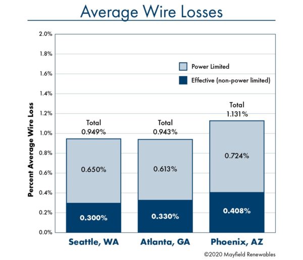
Figure 2: Effective vs. total wire losses across each of our modeled sites (2020 data)
Deconstructing our voltage-drop calculation formula (shown above) we find that the conductor length, current, and source voltage are all variables we can change in our design. Taking a step back and comparing typical values from five to 10 years ago with current standards, we can already start to see why concern for voltage drop is less relevant. System voltages of 600V have been replaced with 1000V and 1500V. Holding all system variables equal, a change from 600V to 1000-1500V could represent a theoretical gain of 40-60% of the voltage lost. To a lesser degree, current has also increased as module technology has improved, but its effect on DC voltage drop is greatly outweighed by the massive leap in system voltage. Cable length has not changed much as it is system-dependent.
Another important factor to consider is power limiting, where the DC input is higher than what the inverters can convert to their rated output, thus the excess DC is essentially lost. Power losses (P=IV) are overcome by the relative cheapness of today’s PV modules and the deal structures utility project EPCs strike with off-takers. In these situations, any voltage loss can be ignored as the system is already limiting the DC input. For example, one of our Atlanta models experienced 589 hours each year in which the array was power-limiting. These decrease the effective losses due to voltage drop. Simply put, the maximum power is delivered regardless of any losses behind the inverter. The customer is happy and the designer did not have to worry about upsizing based on an antiquated rule.
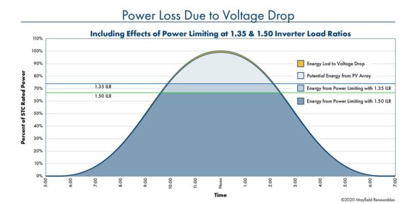
Note: When power limiting, DC voltage drop at peak production hours goes unseen
Voltage Drop Implications
Based on our analysis, it’s clear that a significant gap exists between the assumed 2% DC voltage drop rule, static DC voltage drop calculations using STC, and real-world effective DC power losses. What are the implications of this?
First and foremost, the antiquated 2% DC voltage drop assumption should be rethought. Our analysis shows that this long-held rule of thumb no longer applies to most commercial and utility-scale PV projects. As system voltages and ILRs have increased, the magnitude and importance of DC voltage drop has faded. Perhaps it’s better to reduce the assumed percentage by half. Perhaps it’s better to eliminate the rule entirely and determine wire losses on a site-by-site basis. Either way, system designers can avoid defaulting to 2% DC voltage drop and instead opt for a more accurate estimate.
Secondly, DC voltage drop can be largely ignored in power limiting scenarios typical for PV systems with high ILRs. As is shown in our analysis, power limiting effectively curtails peak system production below the levels with the highest voltage drop. The highest effective (non-power-limited) wire loss we found in our analysis was 0.591%, and the average across all of our test sites was 0.346%. Thus, as power limiting increases, attention given to voltage drop should decrease, and designers and engineers should predominantly focus on non-power-limited hours when analyzing wire losses.
Third, be wary when relying on STC figures for system calculations. Most equipment power ratings will be listed at STC. Although referred to as “standard” they are, in most cases, “ideal” conditions that are not necessarily reflective of real-world operating scenarios. As was noted in our analysis, even in Phoenix, a notoriously sunny climate, only 3% of daylight hours reached STC-levels of irradiance (1000W/m2 ). This dropped to 0.47% of daylight hours in Atlanta and only 0.11% in Seattle. In other words, a simplified voltage drop analysis using STC current rather than simulated current based on historical weather data would have led to less accurate voltage drop estimates.
Lastly, it may be in system designers’ best interest to start with Code-minimum wiring, then model systems to get a sense of the actual DC voltage loss under normal operating conditions. Our Helioscope analysis was fairly quick and painless. We suspect that, in many cases, modeling will show that code-minimum wiring will be sufficient to keep DC voltage drop under 2%, reducing design complexity and minimizing project costs.
***
Originally published on the Mayfield Renewables blog and authored by Ryan Mayfield, Lucas Miller & Nicky van Almelo.
The views and opinions expressed in this article are the author’s own, and do not necessarily reflect those held by pv magazine.
This content is protected by copyright and may not be reused. If you want to cooperate with us and would like to reuse some of our content, please contact: editors@pv-magazine.com.


after 15 years within the PV industry in the UK, My opinion is to stick to good industry practice and leave headroom in the calcs to avoid all voltage drops.
Too much emphasis on the commercial aspect and not enough emphasis on the engineering has caused many issues. Designs right on the edge of minimum voltage loss yet with differing and somewhat unseasonal weather incident’s, I take the approach of cover all possible scenarios.
Where 4mm string cable is common place, use 6mm or 10mm. Its pennies extra but minimises loss and maintains current stability especially we we are starting to install bi facials. I recently installed a 2 kwp bi facial 5 deg westerly tilt in my garden. Panel specifics were 9.5 amp closed circuit yet I have been regularly measuring 12. 4A !! UK STC factor 1.25 my feelings is for bi facials it should be 1.6- 1.8
If concidering MPPT topography, volt drop at the inverter will create an MPPT voltage out of sinc with the actual string voltage~ 2% of a 800V design = 16V. I suppose this is more of a question, but the “knee” point on the IV curve the inverter is using is incorrect ie not the actual max point of the actual string output? if so, larger volt-drop = larger miss-match. Electrical losses generally arive in heat output and degragation factors for components.